Hydrology model

How does the hydrological model work?

The river forecast model predicts streamflow in units of volumetric discharge rate normalized to catchment area (mm/day), which are then converted to a volumetric flow rate in cubic feet per second (cfs). The model is conceptually similar to a traditional rainfall-runoff model, or lumped catchment model, in that it is run over individual watersheds for each different prediction point along a river reach. The model produces daily outputs that represent the probability of streamflow in a given river reach each day over a seven day forecast horizon (i.e., up to seven days in advance). Daily deterministic forecasts are drawn as the median (50th percentile) of the predicted probability distributions.

Model data

Input data to the hydrology model are described in more detail below, but fundamentally consist of three types:

Static catchment attributes representing catchment-wide statistics (e.g., mean, mode, min, max) of several geographical and geophysical variables.
Historical meteorological time series data, including precipitation, temperature, and several other variables.
Forecasted meteorological time series over the seven-day forecast horizon.

All of the data that we currently use to train and test the hydrology model is publicly available, and all data except meteorological forecasts are freely available (i.e., without monetary charge). This means, in principle, all of our modeling results are reproducible and verifiable. One of the meteorological forecast data that we use comes from the ECMWF Integrated Forecast System, and obtaining this data in real time requires a paid license from ECMWF.

Target data: The hydrology model is trained on publicly available historical data mainly from the Global Runoff Data Center and the Caravan dataset.

Static attributes: Geophysical and geographical data are provided to the model as inputs. These come largely from the HydroAtlas dataset, which is part of the HydroSheds project. These include variables about climate, land use and land cover, soils, and human impacts. A full list of the static attributes that we use is available on request. These data are scaler (single) values representing aggregation (fractional coverage, mean, mode, max, etc.) over a given (sub)watershed.

Meteorological data: The hydrology model uses one year of historical meteorological data to spin up to present conditions at the issue time of a forecast, and 7 days of forecasted meteorological data. Meteorological data comes from five sources:

ECMWF HRES Forecast System Meteorological Forecast Data: Daily-aggregated single-level forecasts from the ECMWF Integrated Forecast System High Resolution atmospheric model. Variables include total precipitation (TP), 2-meter temperature (T2M), surface net solar radiation (SSR), surface net thermal radiation (STR), snowfall (SF), and surface pressure (SP). We use data from 2014 - Present.
ECMWF ERA5-Land Meteorological Reanalysis Data: The same six variables as from the IFS-HRES system (listed above), but from the ECMWF ERA5-Land reanalysis. We use data from 1980 - Present.
NASA’s Integrated Multi-satellitE Retrievals for GPM (IMERG) Precipitation Data: Global, gridded precipitation estimates from two satellite platforms: TRMM (2000 - 2015) and GPM (2012 - Present).
NOAA CPC Global Unified Gauge-Based Analysis of Daily Precipitation Data: Global, gridded precipitation data from rain interpolated rain gauges. We use data from 1980 - Present.
GDM AI-based global weather forecasting model (published in Science in 2023)

Is data provided by governments? Unless otherwise stated, the models do not use real-time data provided by governmental entities, nor is Google Flood Forecasting project affiliated with, sponsored by, or endorsed by any governmental entity.

Model structure

The model is based on Long-Short Term Memory networks (LSTMs), which are a type of ML model that operate sequentially over time series data. They use neural networks to define a “transfer function” that is applied at each timestep of a time series prediction task. At each timestep, the transfer function takes as input a state vector from the previous timestep and new inputs for the current timestep, and produces as output a state vector for the current timestep. The state vector for the current time step is used to estimate streamflow at the current timestep. This concept is illustrated in the figure below, and a deeper discussion about conceptual similarities between LSTMs and traditional hydrology models can be found in this paper.

A diagram of the LSTM, which is a neural network that operates sequentially in time. An accessible primer can be found here.

Inputs for every time step include a concatenation of the meteorological input data for that timestep (either historical or forecasted) plus static catchment attributes that we assume do not change in time (loosening this assumption is the subject of future research). These static and dynamic inputs are concatenated with the LSTM state vector from the previous time step and this entire concatenated vector is fed into a series of neural network layers within the LSTM model structure.

The neural networks that make up an LSTM transfer function do two primary tasks: (1) they change the value of the state vector, effectively changing the state of the system based on current inputs, and (2) they predict the output based on the current state and current inputs. In our case the output is a probability distribution over streamflow.

There are three neural network “gates” in the LSTM: the forget gate, the input gate, and the output gate. The forget gate uses concatenated inputs (dynamic inputs, static inputs, and the LSTM state from the previous timestep) to predict a set of attenuation weights (real-valued numbers between 0 and 1) that are multiplied with the current state vector at the beginning of a timestep. This attenuates the values of the state vector and effectively controls the memory timescales of the model. The input gate predicts a set of values that add to the state vector, effectively changing the state of the system based on current inputs. The output gate translates the state vector into output values that are used to make streamflow predictions. All of these gates control effectively nonlinear functions, meaning that the LSTM itself is a nonlinear function.

Before all weather forcing data is fed into an LSTM network, Google’s streamflow forecast model embeds each weather product using its own embedding network. The outputs of the different embedding networks are combined given the data availability, which makes the model robust to individual weather products that might be missing in the operational setting. The output of the LSTM is used to derive the discharge forecasts using a mixture of density networks. We use a countable mixture of asymmetric Laplacians (CMAL) distribution, which represents a probabilistic prediction of the streamflow in a particular river at a particular time (more details below).

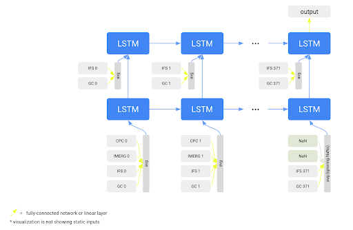
Each weather product is embedded by a different network. The output of all embedding networks are combined and fed into an LSTM network, which outputs the parameters of a probability distribution over streamflow. GC stands for Graphcast.

The first 365 time steps are the hindcast part of the LSTM. It runs sequentially over one year (365 days) of historical weather data, up to the issue time of a current forecast (up to today). The output of this model does not represent streamflow directly, but is an embedding vector (meaning, simply, a vector of numbers) that represents the current state of the system and is updated after each timestep of historical weather data. The subsequent 7 time steps are the forecast part of the LSTM. They take as input only forecast meteorological data from the current day to produce daily streamflow forecasts over the next seven days.

Probabilistic forecasts

The ML hydrology model is probabilistic in the sense that instead of producing estimates of streamflow directly, it predicts parameters of a probability distribution over streamflow, following the methodology outlined in this paper. The predicted probability parameters are different at every timestep, meaning that the probabilistic predictions are different at every timestep.

The model predicts the parameters of an asymmetric Lapacian distribution, which is heavy-tailed to capture the fact that streamflow uncertainty is typically heavy-tailed toward high streamflow values (see the paper for a description of this probability density function). The training loss function is the (analytical) negative log likelihood function of the parameterized asymmetric Laplacian.

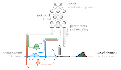
Illustration of how a mixture distribution is predicted from forecast LSTM output.

Streamflow hydrographs shown on Flood Hub represent the median values from the timeseries of predicted probability distributions.

Hydrology model training

The hydrology model is trained using streamflow data mainly from the Global Runoff Data Center and the Caravan dataset over the time period 1980 - 2023. We use training data from approximately 16,000 streamflow gauges, illustrated in the figure below. These locations represent watersheds ranging from 2 km2 to over 4,000,000 km2. We use data from all sizes of watersheds to train a single model.

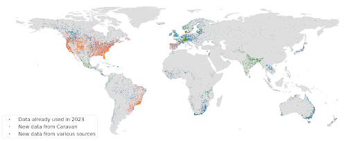
Location of nearly 16000 streamflow gauges that supplied training data mainly from the Global Runoff Data Center and the Caravan dataset.

Notice that not all input data is available for the whole training period (1980 - 2023). In cases where a certain data product is missing we either mask or impute the missing data. ECMWF HRES forecast data is imputed with the corresponding ERA5-Land variable during the time period 1980 - 2012. Missing data from IMERG or CPC is masked, meaning that the actual missing value is imputed with a dummy value (either zero or the overall mean of the dataset), and then a binary flag is fed as an extra input into the model that signals whether the data is real or masked.

As mentioned above, the model is trained using a negative log-likelihood loss function. Other hyperparameters of the model (being quite numerous) are available on request. No part of the model architecture or training procedure is proprietary.

Hydrological model performance

Various versions of LSTM-based streamflow models have been benchmarked extensively in peer-reviewed publications. For example, this paper compares the performance of an LSTM-based simulation (not forecast) model over watersheds in the continental US with several commonly-used research models. This paper compares a simulation LSTM against the two hydrology models that are run operationally for flood forecasting in the United States.

The most up-to-date peer-reviewed model performance statistics can be found in this paper. That paper compares the skill of the Global Flood Awareness System (GloFAS) with Google’s previous hydrology model at predicting the timing of extreme events (1, 2, 5 ,and 10-year return period events). The Google model shows better performance, on average, in all continents, and we achieve either better or statistically indistinguishable performance at five-day lead times as GloFAS achieves over nowcasts (zero-day lead times) – see figure below.

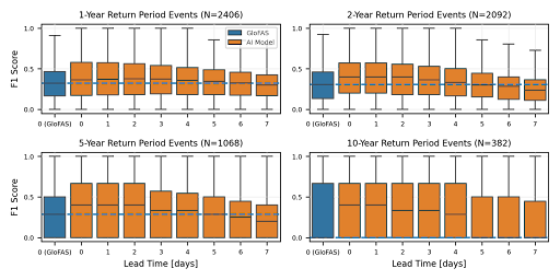
Illustration of reliability over 1, 2, 5, and 10-year return period events in several hundreds of river reaches globally with different lead times, benchmarked against GloFAS. From this paper.

Our new model extends the reliability of global nowcasts to 7 days (as opposed to 5 days) globally.

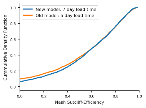
Floods_Forecasting_Hydrologic-density-graph

Cumulative distribution function of the R-square metric for the new model at a 7-day lead time and the previous model at a 5-day lead time (red dashed line), as evaluated on 3079 basins.

Reliability in ungauged basins

A longstanding challenge in hydrology is the problem of Prediction in Ungauged Basins (PUB). This refers to making streamflow predictions in river reaches where there is no streamflow data for calibrating models. ML hydrology models are able to transfer (learned) information between different watersheds and are significantly more reliable in ungauged catchments than other types of hydrology models. This is one of the main reasons why we use an ML-based modeling approach in the Google flood forecasting system. More information, including benchmarks against two hydrolog models used operationally in the United States, can be found in this paper.